Saturday, April 30, 2011

Layton Power: How leadership mattered in the Canadian politics

The rise of NDP is a testament to the star power of Jack Layton, the NDP’s charismatic leader. Where Stephen Harper of Conservatives and Michael Ignatieff of Liberals lagged, Jack Layton lead with style. The issue-less campaign has been galvanized by Mr. Layton and it is paying off handsomely for him. 

This perhaps has been the best April of Mr. Layton’s life who surpassed the prime minister in popularity by mid April (see the graph below). An analysis of the web searches conducted using Google from computers located within Canada suggest that Mr. Layton bypassed his competition as of April 13, a day after his stellar performance in the televised debate in English language with the three other party leaders.

While many political pundits did not find the leaders’ debate as a game changer, the graph below suggests otherwise. Mr. Layton did change the game in his two-hour performance on the television. Since April 21, he has been in a comfortable lead over others.

If there were an Emmy for televised political performance, Jack Layton would have won it hands (and one hip) down.

Saturday, April 23, 2011

US leading indicators improve

The numbers are in and they look good. According to the latest economic stats, the US economy is showing signs of recover. The on-again, off-again recovery in the US has kept the global economic pundits on the fence. So far, extreme scenario forecasters suggesting a complete rebound or an economic Armageddon have been proven wrong. Leading indicators were up 0.4% in March. Earlier in February, the leading indicators were up by 1.0%.
The Conference Board reported that its Index of Leading Economic Indicators rose 0.4% in March after an upwardly revised February gain of 1.0%, originally reported at 0.8%. Consensus expectations were for a 0.3% increase during last month. The latest was the ninth consecutive monthly increase. The three-month growth in the series of 6.6% (AR) was down from its early-2010 high of 10.8%.

Read more on Haver Analytics.
Enhanced by Zemanta

Sunday, April 17, 2011

Business majors spend less time preparing for class-NYTimes.Com

The Default Major - Skating Through B-School - NYTimes.com

Business majors spend less time preparing for class than do students in any other broad field, according to the most recent National Survey of Student Engagement: nearly half of seniors majoring in business say they spend fewer than 11 hours a week studying outside class. In their new book “Academically Adrift: Limited Learning on College Campuses,” the sociologists Richard Arum and Josipa Roksa report that business majors had the weakest gains during the first two years of college on a national test of writing and reasoning skills. And when business students take the GMAT, the entry examination for M.B.A. programs, they score lower than students in every other major.

This is not a small corner of academe. The family of majors under the business umbrella — including finance, accounting, marketing, management and “general business” — accounts for just over 20 percent, or more than 325,000, of all bachelor’s degrees awarded annually in the United States, making it the most popular field of study.

Brand-name programs — the Wharton School of the University of Pennsylvania, the University of Notre Dame Mendoza College of Business, and a few dozen others — are full of students pulling 70-hour weeks, if only to impress the elite finance and consulting firms they aspire to join. But get much below BusinessWeek’s top 50, and you’ll hear pervasive anxiety about student apathy, especially in “soft” fields like management and marketing, which account for the majority of business majors.

Going over the speed limit

In an earlier post [Speeding tickets for R and Stata]  I had reported on how R compared with Stata for executing algorithms involving maximum likelihood estimation. This post  offers the following updates on the last post:

  • Stata is in fact even faster than previously reported.
  • The 64-bit version of the newly released R 2.13.0 reports faster times than the 32-bit version for R 2.12.0.
  • Limdep/NLogit, a popular econometrics software amongst discrete choice modellers, reported slower execution times than R 2.13 (64-bit version).
  • Advice on speed from experienced R users.

    My data set (used for the test results reported below) comprised an ordinal dependant variable [5 categories] and categorical explanatory variables with 63,122 observations. I used a computer running Windows 7 Professional on Intel Core 2 Quad CPU Q9300 @ 2.5 GHz with 8 GB of RAM. Further details about the tests are listed in the following Table.

    Software Routines

    Stata 11 (duo core)

    R (2.12.0) [32-bit]

    R x64 2.13.0

    NLogit/Limdep

    Commercial license price

    US$2,495 Free Free $1,395

    Multinomial Logit

    mlogit, 9.06 seconds 
       (2.89 seconds with 
       the “quietly” option")
    multinom, 50.59 sec + 52.29 sec
    zelig (mlogit), 77.89 sec
    VGLM (multinomial), 64.4 sec
    multinom, 32.7 sec + 49.8 sec
    zelig (mlogit), 69.92 sec
    VGLM (multinomial), 63.76 sec
    Logit; 36.72 sec

    Proportional odds model

    ologit, 1.69 sec
              0.91 sec [quietly]
    oprobit, 0.91 sec [quietly]
    VGLM (parallel = T), 16.26 sec
    polr, 22.62 sec [o.logit]
    VGLM (parallel = T), 14.94 sec
    polr, 13.49 sec [o.logit]
    polr, 14.94 sec [o.probit]
    Ordered [Logit] 18.50 sec
    Ordered [Probit] 36.33 sec

    Generalized Logit

    gologit2, 18.67 sec
    (15.1 seconds with 
       the “quietly” option")
    VGLM (parallel = F), 64.71 sec
    VGLM (parallel = F),  64.86 sec


    Stata is even faster

    When I reran the models using the quietly option (which supresses terminal output ) in Stata, I obtained the actual algorithm convergence times. For the multinomial logit model, Stata took fewer than 3 seconds to converge, making it 10-times faster than R. Similar reductions in execution times for Stata were observed for other algorithms reported in the table above.

    64-bit version of R is faster, sometimes

    The 64-bit version of R (2.13.0) reported faster execution times. The same was observed for the 64-bit version of R (2.12.0). Notice in the table above the dramatic reduction in the convergence times for the multinomial logit model (using multinom). R 2.13.0 [64-bit] took 35.4% less time to converge than R 2.12.0 [32-bit]. However, Zelig and VGLM based algorithms reported very modest improvements in execution times.

    The ordered logit and ordered probit models (executed using the polr algorithm) also reported significant improvements in execution times.The ordered logit model took 40.3% less time in converging for R 2.13.0 [64-bit] than R 2.12.0 [32-bit].

    I still do not understand why the summary(multinomial logit model) still takes an additional 49.8 seconds on top of 32.7 seconds to report summary results for the multinomial logit model. When I do not use summary() and instead use coef(multinomial logit model), I get instantaneous output.

    In summary, it appears that not all algorithms would converge faster in the updated 64-bit version of R 2.13.0.

    R is faster than Limdep/NLogit

    In comparison, R [2.13.0] offered faster convergence times than NLogit for multinomial and ordered logit models and for ordered probit models. This puts R in the middle of two popular econometrics software. Stata is significantly faster than R, and R offers faster execution times than NLogit (see the difference for ordered logit in the table above).

    What R Pros are saying about my post

    If you were to scroll down to the comments section of my last post [Speeding tickets for R and Stata], you’ll notice some advice from experienced users of R. I have been advised to re-run the tests by first obtaining the optimised version of BLAS and LAPACK libraries.  I am not sure how much difference would that make. However, it would be a little difficult for ordinary users of R (such as myself) to be able to determine what BLAS and LAPACK libraries to choose and install that are appropriate for their computer systems.

    If significant speed gains could be achieved by using optimised BLAS and LAPACK libraries, the R installation routines may then be improved so that these libraries are made available to the novice end users of R.

  • Saturday, April 16, 2011

    New Economists Scour Urban Data for Trends - WSJ.com

    Ted Egan, chief economist in the San Francisco Controller's Office, said he could wait six months for California to release the detailed sales-tax data he needs for city revenue projections. But it's quicker to look at passenger tallies from the station closest to the Union Square shopping district, which generates roughly 10% of the city's sales-tax revenue. The Bay Area Rapid Transit District releases the data within three days, he said: "Why should I have to wait?"


    New Economists Scour Urban Data for Trends - WSJ.com

    Friday, April 15, 2011

    Hungry for justice

    From the Economist:

    imageA paper in the Proceedings of the National Academy of Sciences describes how Shai Danziger of Ben-Gurion University of the Negev and his colleagues followed eight Israeli judges for ten months as they ruled on over 1,000 applications made by prisoners to parole boards. The plaintiffs were asking either to be allowed out on parole or to have the conditions of their incarceration changed. The team found that, at the start of the day, the judges granted around two-thirds of the applications before them. As the hours passed, that number fell sharply (see chart), eventually reaching zero. But clemency returned after each of two daily breaks, during which the judges retired for food. The approval rate shot back up to near its original value, before falling again as the day wore on.

    Enhanced by Zemanta

    Thursday, April 14, 2011

    Don't kill yourself on poor economic news

    Suicides rise and fall with economy: CDC report - Yahoo! News

    CHICAGO (Reuters) – Suicides in the United States ebb and flow with the economy, rising in bad times and falling in good, researchers at the Centers for Disease Control and Prevention said on Thursday.

    When you're buying a home, hassle for a better price

    Real Estate = Big MoneyImage by thinkpanama via FlickrFrom The Toronto Star, Wednesday, April 3, 2011

    "At this point, Ryerson University professor Murtaza Haider, who is also the director of the Institute of Housing and Mobility, recommends writing down a reserve price you’ve decided you are comfortable with on a piece of paper.

    “Then, under no circumstances, are you to go a dime over,” he says. “Put it in a safe place.” And in that very last half hour of bargaining, when many start to feel panicky and will bid that extra $20,000, take it out and look at it. If you lose the home, another will come along, he says.

    “People get caught up in the moment,” Haider says. “You have to realize there are millions of housing units in Toronto. There are tons of houses to look at.”

    But what exactly causes rational people to make such poor financial choices when it comes to real estate?

    For Haider, it’s partly human nature and partly cultural.

    The process of making an offer can resemble an auction. The excitement and competiveness of a sale can foster overbidding. Small, incremental increases also seem less significant. What’s $5,000 more when you’re talking $400,000 — it’s an easily mentality to slip into.

    There’s also peer pressure, he says. People tend to look at what their friends and family have as a benchmark of status.

    “And then there are cultural aspects too,” he adds. “We’re not a bargaining society. If you were buying a pair of shoes in Mumbai you would spend half an hour negotiating. The only time we negotiate is buying a house and we do a poor job of it. Our lack of experience comes in and that shows.”

    Haider estimates North Americans are paying anywhere between 2 per cent to 5 per cent more for property because of weak bargaining skills. Sometimes, it can come down to embarrassment. A buyer doesn’t want to look cheap in front of their agent, said Haider."

    Spring buying fever is rampant - Moneyville.ca
    Enhanced by Zemanta

    Monday, April 11, 2011

    Speeding tickets for R and Stata

    How fast is R? Is it as fast in executing routines as the other off-the-shelf software, such as Stata? After some comparative experimentation, I found Stata to be 5 to 8  times faster than R.

    For me, speed has not been a concern in the past. I had used R with smaller datasets of roughly 5000 to 10,000 observations and found it to be as fast as other statistical software. More recently, I have been working with still a relatively small-sized data set of 63,122 observations. After realizing that R was very slow in executing the built-in routines for multinomial and ordinal logit models, I ran similar models in Stata with the same data set and found Stata to be much faster than R.

    Before I go any further, I must confess that I did not try to determine ways to improve speed in R by, for instance, choosing  faster converging algorithms. I hope readers would send me comments on how to speed-up execution for the routines I tested in R.

    My data set comprised an ordinal dependant variable [5 categories] and categorical explanatory variables with 63,122 observations. I used a computer running Windows 7 on Intel Core 2 Quad CPU Q9300 @ 2.5 GHz with 8 GB of RAM. Further details about the test are listed in the following Table.

    Software Routine

    Stata 11 (duo core)

    R (2.12.0)

    Multinomial Logit mlogit, 9.06 seconds multinom, 50.59 seconds
    zelig (mlogit), 77.89 sec
    VGLM (multinomial), 64.4 sec
    Proportional odds model ologit, 1.69 sec VGLM (parallel = T), 16.26 sec
    polr, 22.62 seconds
    Generalized Logit gologit2, 18.67 sec VGLM (parallel = F), 64.71 sec

    I first estimated the standard multinomial logit model in R using the multinom routine. R took almost 51 seconds to return the results. The subsequent call to summarise the model took another 52.29 seconds, thus making the total execution time in R to be 103 seconds. Surprised at the slow speed, I tried other options in R to estimate the same model. I first tested mlogit option in Zelig. The execution time was even slower at 78 seconds. I followed up with VGAM package, which returned a slightly better result with 64.4 seconds.

    Other examples listed above suggest similar slower times for R in comparison with Stata.

    What could be the reason for such an order of magnitude difference in speed between R and Stata. I unfortunately don’t have the answer. I do know that Revolution Analytics offers similar performance benchmark comparisons between their version of souped-up R (Revolution R) and the generic R. Revolution R was found to be five to eight times faster than regular R.

    image

    Other performance benchmarks revealed even greater speed differentials between Revolution R and the generic R.

    image

    There must be ways to make routines execute faster in R. A few weeks earlier, Professor John Fox ( a long-time contributor to R and the programmer of the R GUI, R Commander) delivered a guest lecture at the Ted Rogers School of Management in Toronto at the GTA R Users’ Group meeting. His talk focussed on how to program using binary logit model as an example. His code for binary logit was found to be much faster than the one that comes bundled with the GLM in R.

    This makes me wonder: are there ways to make the generic R run faster?

    Thursday, April 7, 2011

    Diversying United States: The melting pot

    Downtown Los Angeles as seen from my American ...Image via WikipediaFINDINGS

    An analysis of data from the 1990, 2000, and 2010 decennial censuses reveals that:
    • New minorities—Hispanics, Asians, and other groups apart from whites, blacks, and American Indians—account for all of the growth among the nation’s child population. From 2000 to 2010, the population of white children nationwide declined by 4.3 million, while the population of Hispanic and Asian children grew by 5.5 million.
    • In almost half of states and nearly one-third of large metro areas, child populations declined in the 2000s. White child populations dropped in 46 states and 86 of the 100 largest metro areas, but gains of new minority children forestalled more widespread overall declines in youth.
    • In areas of the country gaining children, Hispanics accounted for most of that growth. Fully 95 percent of Texas’s child population growth occurred among Hispanics. Los Angeles was the only major metropolitan area to witness a decline in Hispanic children from 2000 to 2010.
    • Ten states and 35 large metro areas now have minority white child populations. Child populations in the Atlanta, Dallas, Orlando, and Phoenix metro areas flipped to “majority minority” by 2010.
    • Segregation levels for black and Hispanic children are higher than for their adult counterparts, despite a general reduction in segregation over the last 10 years. The average black or Hispanic child lives in a neighborhood where whites make up 10 percent less of the population than in the neighborhood of the average black or Hispanic adult.
    • The accelerating growth of new minority children heralds an increasingly diverse future child population and labor force. While this transition presents challenges for America’s social and political systems, it also represents a clear demographic advantage for the nation and its regions versus its developed peers, one which savvy leaders will capitalize upon in the years and decades to come.
    Enhanced by Zemanta

    Global exports surge record 14.5% in 2010

    Exports jumped 14.5 per cent last year – the biggest rise recorded since 1950 – as economies rebounded from the global downturn, the World Trade Organization said Thursday.

    Cross-border trade is expected to recover further in 2011, the WTO said in its annual report. Based on a 3.1-per-cent rise in gross domestic product worldwide, the Geneva-based body predicts exports will grow another 6.5 per cent this year, slightly above the 6 per cent yearly average between 1990 and 2008.


    Global exports surge record 14.5% in 2010 - The Globe and Mail

    Tuesday, April 5, 2011

    Dirty politics with dirty money

    Stephen Harper, Canadian politicianWhen it comes to Quebec, anglophone politicians while wooing francophone votes, would resort to literally throwing money at Quebec voters.  The Conservative Canadian Prime Minister is now talking of a $2.2 billion bribe (disguised as a Quebec-specific tax deal) to Quebec voters just weeks shy of an election. In a previous election, he offered a billion dollar bribe to Quebec voters.

    I remember reading Preston Manning's book in which he complained how Quebec got a preferential treatment every time. I wonder what Mr. Manning thinks of the Conservative Party of today that literally throws money at Quebec to win a parliamentary majority, which will most likely evade Mr. Harper this time as well.

    Unlike Mr. Harper's Conservatives, Quebec voters are smart. They will take the money, but will vote in their self interest that lies elsewhere.

    Harper confident Quebec’s $2-billion HST deal won’t hinder deficit battle - The Globe and Mail
    Enhanced by Zemanta

    Painting a picture of statistical packages

    Imagine you have to analyze text comprising 18,000 words. You have to identify the most commonly cited ideas or words in the text and then present the analysis in a graphic format. There are sophisticated tools out there to help you with this task, but then again there is a tight deadline. You have fewer than five minutes to accomplish the task.

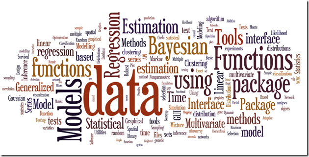
    Generating a word cloud from the text may be one option. It is fast and the resulting output is appealing as well as informative. See the word cloud below, which I have generated from the description of 2,948 R packages listed at http://cran.r-project.org/web/packages. The one-liner description of these packages ran into 18,000-plus words. By using the free word cloud tool Wordle (http://www.wordle.net/), the task was accomplished in less than two minutes.

    image

    Based on the cloud we can see that the most frequent recurring themes in R packages are data, functions, models, estimation, regression, and Bayesian.

    Wordle offers some control over the output. Consider the above cloud that was generated using the most common 150 words in the text. I eliminated ‘Analysis’ from the text since it was the most frequently repeated text. Later, I restricted the cloud to 100 most repeated words and removed restriction on  the word ‘Analysis’, and a randomly generated a word cloud. See the output below.

    image

    Notice the two variants of the word ‘data’ in the cloud. Wordle allows the user to eliminate any word in the generated cloud with a click of a mouse and retain the cleaned version of the cloud.

    Also, don’t miss Drew Conway’s blog on building a more intelligent word clouds at http://www.drewconway.com/zia/?p=2624.

    Monday, April 4, 2011

    African Americans suburbanising in Detroit

    Logo of the American Community Survey, a proje...Image via WikipediaA Dream Still Deferred - NYTimes.com
    AT first glance, the numbers released by the Census Bureau last week showing a precipitous drop in Detroit’s population — 25 percent over the last decade — seem to bear a silver lining: most of those leaving the city are blacks headed to the suburbs, once the refuge of mid-century white flight
    Enhanced by Zemanta

    Friday, April 1, 2011

    R ready to Deduce you

    Despite being one of the most powerful computing platforms, and being free at the same time, R still struggles against other statistical software, such as SPSS and SAS, in gaining mass appeal amongst users of statistical and market intelligence software. Many have cited the absence of a user-friendly graphical user interface (GUI) for R to be partially responsible for its limited success outside the community of dedicated quants.

    A new GUI for R, Deducer, is about to change R’s geeky unfriendly image. Just like R, Deducer is also free and provides the point-and-click ease of a use for R. Deducer is Java-based and therefore provides an avant-garde look and feel that rivals the user-interfaces developed by SAS and SPSS.

    While Deducer is not the first or the only GUI available for R, it is indeed one of the more functional GUIs with the potential for mass appeal. An earlier issue of the journal reviewed R Commander, a popular R GUI, which was developed by Professor John Fox of McMaster University. Deducer is however different from previous attempts to add a user interface to R. First, it is aesthetically pleasing and easy to use with improved interactive dialogue boxes. Second, it is built on newer algorithms coded in R and therefore the output is formatted to meet the every day needs of the analysts. Thirdly, it offers the user interface for the famed R package for graphics, ggplot2, which is fast becoming the gold standard for analytic graphics.

    Deducer has been developed by Ian Fellows, a Ph.D. student in statistics at UCLA, who relied on the functionality already built into JGR, a short for the Java GUI for R. Ian wanted Deducer to be “user friendly enough to be used by someone just starting out, yet flexible and powerful enough to increase the efficiency of expert users.” Deducer comes very close to the objectives set by Ian Fellows.

    Installing Deducer is a three-step process. First, you will have to install a newer version of R[1]. Version 2.12.0 or later is recommended by the developer. The second step involves installing JGR launcher[2]. Once JGR launcher has been installed, run R and install packages JGR and Deducer. You can exit R and launch Deducer from within JGR for future use. Deducer adds additional menus to the JGR user interface for data analysis and graphics. Ian Fellows has developed another package, DeducerExtras, which provides user interfaces for additional statistical routines.

    There is however a one-step installation option available for Windows only. Further details on one-step installation are listed at:

    http://www.deducer.org/pmwiki/pmwiki.php?n=Main.WindowsInstallation
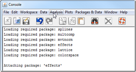
     

    image

    Figure 1

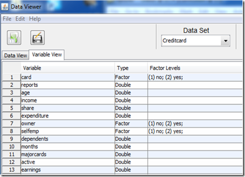
    Users can import data from SPSS, SAS, Stata, DBF, CSV, and other formats in addition to reading data in native R formats. Once the data have been loaded into R, the user can view the data in Data Viewer, which is similar to SPSS and offer two views: data view and the variable view. Data view provides the typical tabular display of data, whereas the variable view presents the Meta data offering details about variable types, and for categorical variables information about factor levels (Figure 2). The variable view is a useful tool to quickly glance through the data to determine how each variable could be used in the analysis. If two or more data sets are loaded, the same data viewer can be deployed to view multiple data sets by selecting the required data set from a dropdown box.
    image

    Figure 2.

    The analysis menu offers the standard analysis tools varying from descriptive statistics and crosstabs to hypothesis testing. On the modelling front, Deducer offers Anova, OLS Regression, Binomial Logit models, and Generalized Linear Models. The advanced add-in package, DeducerExtras, offers further functionality for hypothesis testing and multivariate analysis.

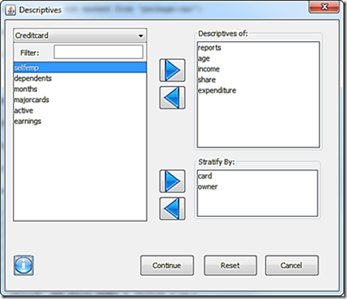
    Deducer offers highly functional dialogue boxes, which also retain in memory choices made in the last deployment. All dialogue boxes in Deducer offer a dropdown menu to select a data set for the analysis, in case two or more data sets are concurrently opened. Variables can be dragged and dropped into the dialogue boxes. Results can be organized by filtering the data as well as using one or more variables to stratify the output.
    image

    Figure 3

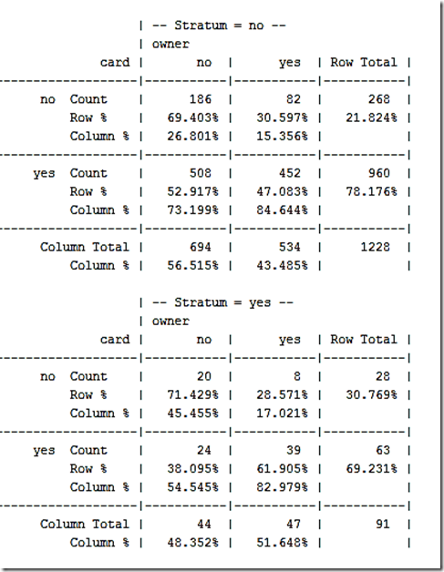
    I illustrate Deducer’s analytic capabilities using a dataset about credit card approvals, which comes embedded in a package in R. Deducer generates output in fixed width text format. A crosstab between two categorical variables, credit card application status and home ownership broken down by a stratification variable, self-employed status, is presented below.
    image

    Figure 4

    Deducer also generates a series of tests to determine the statistical significance of the results obtained from the cross tabulations.

    Deducer’s dialogue boxes for statistical model, such as regression are very similar to those in SPSS. The dialogue box allows the user to introduce explanatory variables either as continuous or categorical variables. Furthermore, the dialogue box also offers the option to create interactions between variables by pointing and clicking. Once the model is specified, Deducer displays the output in another dialogue box so that the analyst may fine tune the model before the results are committed to the output window. This intermediate step of looking at the results on the fly and tweaking the model offers unique interactive functionality in Deducer that is missing in other commercial statistical software.

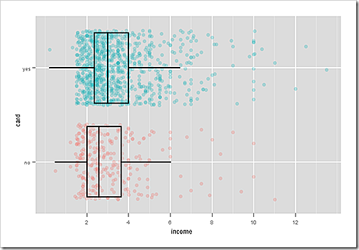
    Deducer’s second most significant feature (its most important feature is it being free) is the interactive user interface for the ggplot (Grammar of Graphics) package. A whole host of graphic templates have been built in to Deducer for the user to develop analytic graphics, which are hard, if not straight out impossible, to create in other commercial statistical software. Apart from the fact that users can create graphics using the plot menu (see Figure 1), Deducer also generates supporting graphs as part of the statistical analysis. For instance, when I conducted the t-test to compare the income of those whose credit card application was successful against those whose application was rejected, Deducer offered the option to visualise the comparison as a box plot (see Figure 5), which it generated using the ggplot package without any additional input from me. This type of functionality in Deducer is of great use to market analysts who could generate supporting results and graphs with minimum input.
    image

    Figure 5

    The numeric output can be saved as text file. Deducer offers the option to save the generated results either with or separate from the R script, which is generated by the dialogue boxes. Thus a user can save the script in a text file to re-run the analysis with modifications by simply highlighting the text and executing it with one click of a mouse.

    Room for improvement

    While Deducer offers dialogue boxes for the most common analytic tasks, it can broaden the scope of analytics by creating user interfaces for algorithms that have already been programmed for R. Another area of improvement is help for its dialogue boxes. Deducer offers on-line help, including text and videos. Deducer should offer off-line text-based help for instances when Internet may not be available to a user.

    Another limitation in Deducer is that it does not retain the results of a statistical routine, such as a regression model, as a temporary object, which could be manipulated later. For instance, one can assign the results from a model to an object, e.g., a variable, and review and manipulate the results later by reviewing the object without executing the model again. However, Deducer removes such temporary objects by default, which may require the analyst to re-run the model from the script. Its dialogue boxes should offer the option to store results as objects for further manipulation.

    I see no reason to keep Deducer and Deducer Extras separate. Currently one has to launch Deducer and DeducerExtras to get the functionality embedded in the two packages. They should be merged so that the user is not required to launch two separate packages every time.

    Final Word

    For businesses and individuals facing tight budgets, Deducer can be a very helpful tool that could be deployed across teams without worrying about hundreds of thousands of dollars in software licensing fees. Deducer has made R as easy to work with as other commercially available software. It is pleasing to look at and generates presentable reports and stunning analytic graphics.


    [1] Download the latest version of R from http://cran.r-project.org/.

    [2] Download JGR launcher from http://rforge.net/JGR/.

    Enhanced by Zemanta

    New York housing prices still depressed

    The reports on the labour market in the US suggest improvement. Job losses have either disappeared or are falling. Still, most housing markets in the US continue to paint a dismal picture. Take New York for instance, where the housing prices started to collapse in 2007. Four years later, the housing prices are still nowhere near their peak in 2007.

    image

    Google maps and travel times

    Travel times and trip distances are at the core of urban economics. Many models of competition, housing markets, etc., rely on travel times or distances to explain the variance in economic outcomes. Determining travel times, especially non free-flow travel times (i.e., accounting for congestion) is however no trivial task.

    Google maps offer a unique opportunity to compute travel times for an origin and destination pair by different modes, i.e., automobile, transit, and walk. The technology is still in Beta stage, but offers realistic travel time estimates for intra-urban trips for many North American cities.

    In the recent Stata journal (Volume 11, No. 1), Adam Ozimek and Daniel Miles highlight their code (now available in Stata) that can not only geocode (determine longitude and latitude) addresses, but also determines travel times by different modes using Google maps.

    I thought R must have some utility already available through CRAN. However, I couldn’t find one. R does offer several interesting spatial analytical capabilities under the Task: Analysis of Spatial Data. However, not much is available on harnessing Google’s analytics to determine distances or travel times. I hope I am wrong and have missed the package that offers these capabilities in R.

    Also worthy of mention is the TravelR project, which is in pre-alpha stage, but once completed will allow R users to develop travel demand models capable of forecasting congested travel times on street networks in addition to other capabilities.  Further details about TavelR are available from Jeremy Raw.