Modern Data Science with R: A review

Some say data is the new oil. Others equate its worth to water. And then there are those who believe that data scientists will be (in fact, they already are) one of the most sought-after workers in knowledge economies.

Millions of data-centric jobs require millions of trained data scientists. However, the installed capacity of graduate and undergraduate programs in data science is nowhere near meeting this demand over the next many years.

So how do we produce data scientists?

Given the enormous demand for data scientists and the fixed supply from higher education institutions, it is quite likely that one must look beyond colleges and universities to train a large number of data scientists desired by the marketplace.

Getting trained on the job is one possible route. This will require repurposing the existing workforce. To prepare the current workforce for data science, one needs training manuals. One such manual is Modern Data Science with R (MDSR).

Published by the CRC Press (Taylor and Francis Group) and authored by three leading academics: Professors Baumer, Kaplan, and Horton, MDSR is the missing manual for data science with R. The book is equally relevant to data science programs in higher ed as it is to practitioners who would like to embark on a career in data science or to get a taste of an aspect of data science that they have not explored in the past.

As the book’s name suggests, the text is based on R, one of the most popular and versatile computing platforms. R is a freeware and is being developed by thousands of volunteers in real time. In addition to base R, which comes bundled with thousands of commands and functions, the user-written packages, whose number has exceeded 14,000 (as of May 2019), further expand the universe of features making R perhaps the most diverse computing platform.

Despite the immense popularity of data science, only a handful of titles focus exclusively on the topic. Hadley Wickham’s R for Data Science and R Cookbook by Paul Teetor are the other two other worthy texts. MDSR is unique in the sense that it serves as an introduction to a whole host of analytic techniques that are seldom covered in one title.

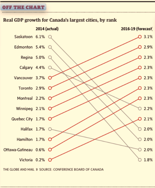
In the following paragraphs, I’ll discuss the salient features of the textbook. I begin with my favourite attribute of the book that deals with its organization. Instead of muddling with theories and philosophies, the book gets straight to business and starts the conversation with data visualization. A graphic is worth a thousand words, and MDSR is proof of it.

And since Hadley Wickham’s influence on data science is ubiquitous, MDSR also embraces Wickham’s implementation of Grammar of Graphics in R with one of the most popular R packages, ggplot2.

Another avenue where Wickham’s influence is widely felt is data wrangling. A suite of R packages bundled under the broader rubric of Tidyverse is influencing how data scientists manipulate small and big data. Chapter 4 in MDSR perhaps is one of the best and succinct introduction to data wrangling with R and Tidyverse. From the simplest to more advanced examples, MDSR equips the beginner with the basics and the advanced user with new ways to think about analyzing data.

A key feature of MDSR is that it’s not another book on statistics or econometrics with R. Yours truly is guilty of authoring one such book. Instead, MDSR is a book focused squarely on data manipulation. The treatment of statistical topics is not absent from the book; however, it’s not the book’s focus. It is for this reason that the discussion on Regression models is in the appendices.

But make no mistake, even when statistics is not the focus, MDSR offers sound advice on the practice of statistics. Section 7.7, The perils of p-values, warns the novice statisticians about not becoming the unsuspecting victims of hypothesis testing.

The books distinguishing feature remains the diversity of data science challenges it addresses. For instance, in addition to data visualization, the book offers an introduction to interactive data graphics and dynamic data visualization.

At the same time, the book covers other diverse topics, such as database management with SQL, working with spatial data, analyzing text-based (non-structured) data, and the analysis of networks. A discussion about ethics in data science is undoubtedly a welcome feature in the book.

The book is punctuated with hundreds of useful and hands-on data science examples and exercise, providing ample opportunities to put concepts to practise. The book’s accompanying website offers additional resources and code examples. At the time of this review, not all code was available for download.

Also, while I was able to reproduce more straightforward examples, I ran into trouble with complex ones. For instance, I could not generate advanced spatial maps showing flights origins and destinations.

My recommendation to authors will be to maintain an active supporting website because R packages are known to evolve, and some functionality may change or disappear over time. For instance, the mapping algorithms that are part of the ggmap package now require a Google maps API or else the maps will not display. This change has likely occurred after the book was published.

In summary, for aspiring and experienced data scientists, Modern Data Science with R is a book deserving to be in their personal libraries.

Murtaza Haider lives in Toronto and teaches in the Department of Real Estate Management at Ryerson University. He is the author of Getting Started with Data Science: Making Sense of Data with Analytics, which was published by the IBM Press/Pearson.

R: simple for complex tasks, complex for simple tasks

When it comes to undertaking complex data science projects, R is the preferred choice for many. Why? Because handling complex tasks is simpler in R than other comparable platforms.

Regrettably, the same is not true for performing simpler tasks, which I would argue is rather complex in base R. Hence, the title -- R: simple for complex tasks, complex for simple tasks.

Consider a simple, yet mandatory, task of generating summary statistics for a research project involving tabular data. In most social science disciplines, summary statistics for continuous variables require generating mean, standard deviation, number of observations, and perhaps minimum and maximum. One would have hoped to see a function in base R to generate such table. But there isn’t one.

Of course, several user-written packages, such as psyche, can generate descriptive statistics in a tabular format. However, this requires one to have advanced knowledge of R and the capabilities hidden in specialized packages whose number now exceed 12,000 (as of March 2018). Keeping abreast of the functionality embedded in user-written packages is time-consuming.

Some would argue that the summary command in base R is an option. I humbly disagree.

First, the output from summary is not in a tabular format that one could just copy and paste into a document. It would require significant processing before a simple table with summary statistics for more than one continuous variable could be generated. Second, summary command does not report standard deviation.

I teach business analytics to undergraduate and MBA students. While business students need to know statistics, they are not studying to become statisticians. Their goal in life is to be informed and proficient consumers of statistical analysis.

So, imagine an undergraduate class with 150 students learning to generate a simple table that reports summary statistics for more than one continuous variable. The simple task requires knowledge of several R commands. By the time one teaches these commands to students, most have made up their mind to do the analysis in Microsoft Excel instead.

Had there been a simple command to generate descriptive statistics in base R, this would not be a challenge for instructors trying to bring thousands more into R’s fold.

In the following paragraphs, I will illustrate the challenge with an example and identify an R package that generates a simple table of descriptive statistics.

I use mtcars dataset, which is available with R. The following commands load the dataset and display the first few observations with all the variables.

data(mtcars)

head(mtcars)

As stated earlier, one can use summary command to produce descriptive statistics.

summary(mtcars)

Let’s say one would like to generate descriptive statistics including mean, standard deviation, and the number of observations for the following continuous variables: mpg, disp, and hp. One can use the sapply command and generate the three statistics separately and combined them later using the cbind command.

The following command will create a vector of means.

mean.cars = with(mtcars, sapply(mtcars[c("mpg", "disp",  "hp")], mean))

Note that the above syntax requires someone learning R to know the following:

1.    Either to attach the dataset or to use with command so that sapply could recognize variables.

2.    Knowledge of subsetting variables in R

3.    Familiarity with c to combine variables

4.    Being aware of enclosing variable names in quotes

We can use similar syntax to determine standard deviation and the number of observations.

sd.cars = with(mtcars, sapply(mtcars[c("mpg", "disp",  "hp")], sd)); sd.cars

n.cars = with(mtcars, sapply(mtcars[c("mpg", "disp",  "hp")], length)); n.cars

Note that the user needs to know that the command for number of observations is length and for standard deviation is sd.

Once we have the three vectors, we can combine them using cbind that generates the following table.

cbind(n.cars, mean.cars, sd.cars)

     n.cars mean.cars    sd.cars

mpg      32  20.09062   6.026948

disp     32 230.72188 123.938694

hp       32 146.68750  68.562868

Again, one needs to know the round command to restrict the output to a specific number of decimals. See below the output with two decimal points.

round(cbind(n.cars, mean.cars, sd.cars),2)

     n.cars mean.cars sd.cars

mpg      32     20.09    6.03

disp     32    230.72  123.94

hp       32    146.69   68.56

One can indeed use a custom function to generate the same with one command. See below.

round(with(mtcars, t(sapply(mtcars[c("mpg", "disp",  "hp")],

                    function(x) c(n=length(x), avg=mean(x),

                    stdev=sd(x))))), 2)

      n    avg  stdev

mpg  32  20.09   6.03

disp 32 230.72 123.94

hp   32 146.69  68.56

But the question I have for my fellow instructors is the following. How likely is an undergraduate student taking an introductory course in statistical analysis to be enthused about R if the simplest of the tasks need multiple lines of codes? A simple function in base R could keep students focussed on interpreting data rather than worrying about missing a comma or a parenthesis.

stargazer* is an R package that simplifies this task. Here is the output from stargazer.

library(stargazer)

stargazer(mtcars[c("mpg", "disp",  "hp")], type="text")

============================================
Statistic N   Mean   St. Dev.  Min     Max  
--------------------------------------------
mpg       32 20.091   6.027   10.400 33.900 
disp      32 230.722 123.939  71.100 472.000
hp        32 146.688  68.563    52     335  
--------------------------------------------

A simple task, I argue, should be accomplished simply. My plea will be to include in base R a simple command that may generate the above table with a command as simple as the one below:

descriptives(mpg, disp, hp)

*  Hlavac, Marek (2015). stargazer: Well-Formatted Regression and Summary Statistics Tables.  R package version 5.2. http://CRAN.R-project.org/package=stargazer

Is it time to ditch the Comparison of Means (T) Test?

For over a century, academics have been teaching the Student’s T-test and practitioners have been running it to determine if the mean values of a variable for two groups were statistically different.

It is time to ditch the Comparison of Means (T) Test and rely instead on the ordinary least squares (OLS) Regression.

My motivation for this suggestion is to reduce the learning burden on non-statisticians whose goal is to find a reliable answer to their research question. The current practice is to devote a considerable amount of teaching and learning effort on statistical tests that are redundant in the presence of disaggregate data sets and readily available tools to estimate Regression models.

Before I proceed any further, I must confess that I remain a huge fan of William Sealy Gosset who introduced the T-statistic in 1908. He excelled in intellect and academic generosity. Mr. Gosset published the very paper that introduced the t-statistic under a pseudonym, the Student. To this day, the T-test is known as the Student’s T-test.   

My plea is to replace the Comparison of Means (T-test) with OLS Regression, which of course relies on the T-test. So, I am not necessarily asking for ditching the T-test but instead asking to replace the Comparison of Means Test with OLS Regression.

The following are my reasons:

1.       Pedagogy related reasons:

a.       Teaching Regression instead of other intermediary tests will save instructors considerable time that could be used to illustrate the same concepts with examples using Regression.

b.       Given that there are fewer than 39 hours of lecture time available in a single semester introductory course on applied statistics, much of the course is consumed in covering statistical tests that would be redundant if one were to introduce Regression models sooner in the course.

c.        Academic textbooks for undergraduate students in business, geography, psychology dedicate huge sections to a battery of tests that are redundant in the presence of Regression models.

                                                               i.      Consider the widely used textbook Business Statistics by Ken Black that requires students and instructors to leaf through 500 pages before OLS Regression is introduced.

                                                             ii.      The learning requirements of undergraduate and graduate students not enrolled in economics, mathematics, or statistics programs are quite different. Yet most textbooks and courses attempt to turn all students into professional statisticians.

2.       Applied Analytics reasons

a.       OLS Regression model with a continuous dependent variable and a dichotomous explanatory variable produces the exact same output as the standard Comparison of Means Test.

b.       Extending the comparison to more than two groups is a straightforward extension in Regression where the dependent variable will comprise more than two groups.

                                                               i.      In the tradition statistics teaching approach, one advises students that the T-test is not valid to compare the means for more than two groups and that we must switch to learning a new method, ANOVA.

                                                             ii.      You might have caught on my drift that I am also proposing to replace teaching ANOVA in introductory statistics courses with OLS Regression.

c.        A Comparison of Means Test illustrated as a Regression model is much easier to explain than explaining the output from a conventional T-test.

After introducing Normal and T-distributions, I would, therefore, argue that instructors should jump straight to Regression models.

 Is Regression a valid substitute for T-tests?

In the following lines, I will illustrate that the output generated by OLS Regression models and a Comparison of Means test are identical. I will illustrate examples using Stata and R.

Dataset

I will use Professor Daniel Hamermesh’s data on teaching ratings to illustrate the concepts. In a popular paper, Professor Hamermesh and Amy Parker explore whether good looking professors receive higher teaching evaluations. The dataset comprises teaching evaluation score, beauty score, and instructor/course related metrics for 463 courses and is available for download in R, Stata, and Excel formats at: 

https://sites.google.com/site/statsr4us/intro/software/rcmdr-1

Hypothetically Speaking

Let us test the hypothesis that the average beauty score for male and female instructors is statistically different. The average (normalized) beauty score for male instructors was -0.084 for male instructors and 0.116 for female instructors. The following Box Plot illustrates the difference in beauty scores. The question we would like to answer is whether this apparent difference is statistically significant.

I first illustrate the Comparison of Means Test and OLS Regression assuming Equal Variances in Stata.

 Assuming Equal Variances (Stata)

Download data

       use "https://sites.google.com/site/statsr4us/intro/software/rcmdr-1/teachingratings.dta"

encode gender, gen(sex) // To convert a character variable into a numeric variable.

The T-test is conducted using:

       ttest beauty, by(sex)

The above generates the following output:

As per the above estimates, the average beauty score of female instructors is 0.2 points higher and the t-test value is 2.7209. We can generate the same output by running an OLS regression model using the following command:

reg beauty i.sex

The regression model output is presented below.

Note that the average beauty score for male instructors is -0.2 points lower than that of females and the associated standard errors and t-values (highlighted in yellow) are identical to the ones reported in the Comparison of Means test. 

Unequal Variances

But what about unequal variances? Let us first conduct the t-test using the following syntax:

ttest beauty, by(sex) unequal

The output is presented below:

Note the slight change in standard error and the associated t-test.

To replicate the same results with a Regression model, we need to run a different Stata command that estimates a variance weighted least squares regression. Using Stata’s vwls command:

vwls beauty i.sex

Note that the last two outputs are identical. 

Repeating the same analysis in R

To download data in R, use the following syntax:

url = "https://sites.google.com/site/statsr4us/intro/software/rcmdr-1/TeachingRatings.rda"

download.file(url,"TeachingRatings.rda")

load("TeachingRatings.rda")

For equal variances, the following syntax is used for T-test and the OLS regression model.

t.test(beauty ~ gender, var.equal=T)

summary(lm(beauty ~ gender))

The above generates the following identical output as Stata.

For unequal variances, we need to install and load the nlme package to run a gls version of the variance weighted least square Regression model.

t.test(beauty ~ gender)

install.packages(“nlme”)

library(nlme)

summary(gls(beauty ~ gender,  weights=varIdent(form = ~ 1 | gender)))

The above generates the following output:

So there we have it, OLS Regression is an excellent substitute for the Comparison of Means test.

The X-Factors: Where 0 means 1

Hadley Wickham in a recent blog post mentioned that "Factors have a bad rap in R because they often turn up when you don’t want them." I believe Factors are an even bigger concern. They not only turn up where you don't want them, but they also turn things around when you don't want them to.

Consider the following example where I present a data set with two variables: x and y. I represent age in years as 'y' and gender as a binary (0/1) variable as 'x' where 1 represents males.

I compute the means for the two variables as follows:

The average age is 43.6 years, and 0.454 suggests that 45.4% of the sample comprises males. So far so good. 

Now let's see what happens when I convert x into a factor variable using the following syntax:

The above code adds a new variable male to the data set, and assigns labels female and male to the categories 0 and 1 respectively.

I compute the average age for males and females as follows:

See what happens when I try to compute the mean for the variable 'male'.

Once you factor a variable, you can't compute statistics such as mean or standard deviation. To do so, you need to declare the factor variable as numeric. I create a new variable gender that converts the male variable to a numeric one.

I recompute the means below. 

Note that the average for males is 1.45 and not 0.45. Why? When we created the factor variable, it turned zeros into ones and ones into twos. Let's look at the data set below:

Several algorithms in R expect the factor variable to be of 0/1 form. If this condition is not satisfied, the command returns an error. For instance, when I try to estimate the logit model with gender as the dependent variable and y as the explanatory variable, R generates the following error:

Factor or no factor, I would prefer my zeros to stay as zeros!

Five Questions about Data Science

From Safari Books Online (https://www.safaribooksonline.com/blog/2016/02/10/data-science-qa/) 

---

Recently, we were able to ask five questions of Murtaza Haider, about the new book from IBM Press called “Getting Started with Data Science: Making Sense of Data with Analytics.” Below, the author talks about the benefits of data science in today’s professional world.

1. What are some examples of data science altering or impacting traditional professional roles already?

Only a few years ago there did not exist a job with the title Chief data scientist. But that was then. Small and large corporations, and increasingly government agencies are putting together teams of data scientists and analysts under the leadership of Chief data scientists. Even White House has a Chief data scientist position, currently held by Dr. DJ Patel.

The traditional role for those who analyzed data was that of a computer programmer or a statistician. In the past, firms collected large amounts of data to archive rather than to subject it to analytics to assist with smart decision-making. Companies did not see value in turning data into insights and instead relied on the gut feeling of managers and anecdotal evidence to make decisions.

Big data and analytics have alerted businesses and governments to the latent potential of turning bits and bytes into profits. To enable this transformation, hundreds of thousands of data scientists and analysts are needed. Recent reports suggest that the shortage of such professionals will be in millions. No wonder we see hundreds of postings for data scientists on LinkedIn.

As businesses increasingly depend upon analytics-driven decision making, data scientists and analysts are simultaneously becoming front-office superstars, which is quite a change from them being the back office workers in the past.

2. What steps can a professional take today to learn how and why to implement data science into their current role?

Sooner than later, workers will find their managers asking them to assume additional responsibilities that would involve dealing with data, and either generating or consuming analytics. Smart professionals, who are uninitiated in data science, would therefore proactively address this shortcoming in their portfolio by acquiring skills in data science and analytics. Fortunately, in the world awash with data, the opportunities to acquire analytic skills are also ubiquitous.

For starters, professionals should consider enrolling in open online courses offered by the likes of Coursera and BigDataUniversity.com. These platforms offer a wide variety of training opportunities for beginners and advanced users of data and analytics. At the same time, most of these offerings are free.

For those professionals who would like to pursue a more structured approach, I suggest that they consider continuing education programs offered by the local universities focusing on data and analytics. While working full-time, the professionals can take part-time courses in data science to fill the gap in their learning and be ready to embrace impending change in their roles.

3. Do you need programming experience to get started in data? What kind of methods and techniques can you utilize in a program more commonly used, such as Excel?

Computer programming skills are a definite plus for data scientists, but they are certainly not a limiting factor that would prevent those trained in other disciplines from joining the world of data scientists. In my book, Getting Started with Data Science, I mentioned examples of individuals who took short courses in data science and programming after graduating from non-empirical disciplines, and subsequently were hired in data scientist roles that paid lucrative salaries.

The choice of analytics tools depends largely on the discipline and the type of organization you are currently working for or intend to work for in the future. If you intend to work for corporations that generate real big data, such as telecom and Internet-based establishments, you need to be proficient in big data tools, such as Spark and Hadoop. If you would like to be employed in the industry that tracks social media, you would require skills in natural language programming and proficiency in languages such as Python. If you happen to be interested in a traditional market research firm, you need proficiency in analytics software, such as SPSS and R.

If your focus is on small and medium size enterprises, proficiency in Excel could be a great asset, which would allow you to deploy its analytics capabilities, such as Pivot Tables, to work with small sized data.

A successful data scientist is one who knows some programming, basic understanding of statistical principles, possesses a curious mind, and is capable of telling great stories. I argue that without the storytelling capabilities, a data scientist will be limited in his or her abilities to become a leader in the field.

4. How do you see data science affecting education and training moving forward? What benefits will it bring to learning at all levels?

Schools, colleges, universities and others involved in education and learning are putting big data and analytics to good use. Universities are crunching large amounts of data to determine what gaps in learning at the high school level act as impediments to success in the future. Schools are improving not just curriculum, but also other strategies to improve learning outcomes. For instance, research in India using large amounts of data showed that when children in low-income communities were offered free meals at school, their dropout rates declined and their academic achievements improved.

Big data and analytics provide instructors and administrators the opportunity to test their hypothesis about what works and what doesn’t in learning, and replace anecdotes with hard evidence to improve pedagogy and learning. Learning has taken a new shape and form with open online courses in all disciplines. These transformative changes in learning have been enabled by advances in information and communication technologies, and the ability to store massive amounts of data.

5. Do you think that modern governments and societies are prepared for what changes that big data and data science might bring to the world?

Change is inevitable. Despite what modern governments and societies like, they would have to embrace change. Fortunately, smart governments and societies have already embraced data-driven decision-making and evidence-based planning. Governments in developing countries are already using data and analytics to devise effective poverty-reducing strategies. Municipal governments in developed economies are using data and advanced analytics to find solutions to traffic congestion. Research in health and well-being is leveraging big data to discover new medicines and cures for illnesses that challenge us all.

As societies embrace data and analytics as tools to engineer prosperity and well-being, our collective abilities to achieve a better tomorrow will be further enhanced.

Getting Started with Data Science: Storytelling with Data

Earlier this month, IBM Press and Pearson have published my book titled: Getting Started with Data Science: Making Sense of Data with Analytics. You can download sample pages, including a complete chapter. There are 104 pages in the sample. You can also watch a brief interview about the book recorded earlier at the IBM Insight2015 Conference.

The very purpose of authoring this book was to rethink the way we have been teaching statistics and analytics to students and practitioners. It is no secret that most students required to take the mandatory stats course dislike it. I believe it has something to do with the way we have been teaching the subject than to do with the aptitude of our students. Furthermore, I believe there is a greater opportunity to equip the students with the skills needed in a world awash with data where competing on analytics defines the real competitive advantage.

No wonder, the latest issue of the leading publication on the subject, The American Statistician, is dedicated to reimagining how statistics should be taught in the undergraduate curriculum. The editors noted:

“We hope that this collection of articles as well as the online discussion provide useful fodder for further review, assessment, and continuous improvement of the undergraduate statistics curriculum that will allow the next generation to take a leadership role by making decisions using data in the increasingly complex world that they will inhabit.”

I am confident that my book will do its small part in equipping the next generation of students with the kind of skills needed to succeed in a data-centric world. For one, I have taken a storytelling approach to statistics. This book reinforces the point that data science and analytics training should be applied rather than theoretical, and the ultimate purpose of producing or consuming statistical analysis is to tell fascinating stories from it. Therefore, the book opens with the chapter titled, The Bazaar of Storytellers.

Who is this book for?

While the world is awash with large volumes of data, inexpensive computing power, and vast amounts of digital storage, the skilled workforce capable of analyzing data and interpreting it is in short supply. A 2011 McKinsey Global Institute report suggests that “the United States alone faces a shortage of 140,000 to 190,000 people with analytical expertise and 1.5 million managers and analysts with the skills to understand and make decisions based on the analysis of big data.”


Getting Started with Data Science (GSDS) is a purpose-written book targeted at those professionals who are tasked with analytics, but they do not have the comfort level needed to be proficient in data-driven analytics. GSDS appeals to those students who are frustrated with the impractical nature of the prescribed textbooks and are looking for an affordable text to serve as a long-term reference. GSDS embraces the 24-7 streaming of data and is structured for those users who have access to data and software of their choice, but do not know what methods to use, how to interpret the results, and most importantly how to communicate findings as reports and presentations in print or on-line.

GSDS is a resource for millions employed in knowledge-driven industries where workers are increasingly expected to facilitate smart decision-making using up-to-date information that sometimes takes the form of continuously updating data.

At the same time, the learning-by-doing approach in the book is equally suited for independent study by senior undergraduate and graduate students who are expected to conduct independent research for their coursework or dissertations.

Praise for the book

I am also pleased to share with you the praise for my book by Dr. Munir Sheikh, Canada’s former chief statistician:

“The power of data, evidence, and analytics in improving decision-making for individuals, businesses, and governments is well known and well documented. However, there is a huge gap in the availability of material for those who should use data, evidence, and analytics but do not know how. This fascinating book plugs this gap, and I highly recommend it to those who know this field and those who want to learn.”

— Munir A. Sheikh, Ph.D., Distinguished Fellow and Adjunct Professor at Queen’s University

Tom Davenport, author of the bestselling books Competing on Analytics and Big Data @ Work.has the following to say about my book:

“A coauthor and I once wrote that data scientists held ‘the sexiest job of the 21st century.’ This was not because of their inherent sex appeal, but because of their scarcity and value to organizations. This book may reduce the scarcity of data scientists, but it will certainly increase their value. It teaches many things, but most importantly it teaches how to tell a story with data.”

—Thomas H. Davenport, Distinguished Professor, Babson College; Research Fellow, MIT.

Dr. Patrick Surry, Chief Data Scientist at www.Hopper.com had the following to say:

“This book addresses the key challenge facing data science today, that of bridging the gap between analytics and business value. Too many writers dive immediately into the details of specific statistical methods or technologies, without focusing on this bigger picture. In contrast, Haider identifies the central role of narrative in delivering real value from big data.

“The successful data scientist has the ability to translate between business goals and statistical approaches, identify appropriate deliverables, and communicate them in a compelling and comprehensible way that drives meaningful action. To paraphrase Tukey, ‘Far better an approximate answer to the right question, than an exact answer to a wrong one.’ Haider’s book never loses sight of this central tenet and uses many realworld examples to guide the reader through the broad range of skills, techniques, and tools needed to succeed in practical data-science. “Highly recommended to anyone looking to get started or broaden their skillset in this fast-growing field.”

And finally, Professor Atif Mian, author of the best-selling book: The House of Debt offered the following assessment:

“We have produced more data in the last two years than all of human history combined. Whether you are in business, government, academia, or journalism, the future belongs to those who can analyze these data intelligently. This book is a superb introduction to data analytics, a must-read for anyone contemplating how to integrate big data into their everyday decision making.”

— Professor Atif Mian, Theodore A. Wells ’29 Professor of Economics and Public Affairs,
Princeton University; Director of the Julis-Rabinowitz Center for Public Policy and Finance at the Woodrow Wilson School.

Not so sweet sixteen!

In the world of big data and real-time analytics, Microsoft users are still living with the constraints of the bygone days of little data and basic numeracy.

If you happen to use Microsoft Excel for running Regressions, you will soon realize your limits:  The Windows version of Excel 2013 permits no more than 16 explanatory variables.

Excel has made great progress in expanding its capabilities in the recent past. Unlike the few thousand rows in the past, the current version permits about a million rows per Sheet (a single data set). But when it comes to regression, you may have several thousand observations in the data set, you are still limited by a hard constraint of sixteen explanatory variables.

Some would argue that for parsimony, we should be content with the restriction. True, but with categorical variables, the number of explanatory variables stretch beyond the artificial constraints set by Microsoft Excel.

Others might inquire why do statistical analyses in Excel in the first place. Despite the inherent limitations in Microsoft Excel, business schools in particular and other social science undergraduate programs in general, are increasingly turning to Excel to teach courses in statistics. If you were to take a quick look at the curriculum of the undergraduate business and numerous MBA programs, you would realize how widespread is the use of Excel for courses in statistics and analytics.

At Ryerson University, I switched to R years ago for my MBA courses. Thanks to John Fox’s R Commander, the transition to R was without much hassle. The students were told in the very beginning that they were now part of the big league, and hiding behind spreadsheets was no longer an option.

I must mention that Microsoft Excel continues to be my platform of choice for a variety of tasks. I use Excel several times a day, but not for statistical analysis. I am not suggesting that Excel cannot do statistics; I am arguing that it can do a much better job of it.

As I see it, Microsoft has several options. First is do nothing. After all, Microsoft Excel has no real competition in the Windows environment. Second, it could turn to the team that has programmed the linest function in Excel and ask them to add some muscle to it. That will be the wrong approach.

Instead, Microsoft should explore ways to integrate R or another freeware with Excel to add a complete analytics menu. Microsoft should learn from what the leaders in analytics are already doing. SPSS, an industry leader in analytics category, has already integrated R, allowing the SPSS users to merge the robust data management strengths of SPSS with the state-of-the-art analytics bundled with R. SAS, another big name in analytics, is about to do the same.

And since Microsoft has recently acquired Revolution R, it makes even more sense to build a bridge between Excel and Revolution R Open (RRO).

R Through Excel is one example of integrating R with Excel. If Microsoft were to put its weight behind the initiative, it could build a seamless coupling with R expanding the analytic capabilities for hundreds of million Excel users.

As for the SPSS, I recommend they also consider another option. If Microsoft were to integrate RRO with Excel, they could acquire an advanced analytics software and integrate it with SPSS. For this option, I would recommend Limdep, which I have found to be the most diverse software for statistical analysis and econometrics. Even though R is a collective effort of thousands of software developers, Limdep offers numerous routines and post-estimation options that are not available in the thousands of R packages. SPSS integrated with Limdep could become the most diversely capable commercial software in the market as it will bridge the gap with SAS and Stata.

As for the colleagues in business faculties pondering over what platform to adopt for the analytics/software courses, I would say know your limits, especially with Microsoft Excel while deciding upon the curriculum.

Curious about big data in Montreal?

Are you in Montreal and curious about big data? Well here is your chance to attend a session about the same at Concordia University on Tuesday, Nov. 03 at 6:00 pm.

www.BigDataUniversity.com, which is an IBM-led initiative is running meetups across North America to create awareness about, and training in, big data analytics.

BigDataUniversity runs MOOCs and through its online data scientist workbench provides access to python, R, and even Spark. Also, you can learn about Watson Analytics and see how you can work with the state-of-the-art in computing.

Further details are available at:

Getting started with Data Science and Introduction to Watson Analytics

http://www.meetup.com/YUL-Social-Mobile-Analytics-Cloud-Meetup/

When: Tuesday, November 3rd at 6-9 PM

Where: H1269, 12th floor of the Hall Bldg 

(1455, blvd. De Maisonneuve ouest - Metro Guy-Concordia)

Are Canadian newspapers painting false pictures with data?

The Canadian newspaper, Globe and Mail, is a leader in diction and style, but it may need improvement in the ‘grammar of graphics’.

Globe’s recent depiction of metropolitan economic growth in the series Off the Charts was way off the mark. The chart plotted the current and forecasted GDP growth rates for select cities in Canada. The red-coloured upward sloping lines depicted cities with increasing economic growth rates and the grey-colored downward sloping lines highlighted those with slowing economic growth.

There is, however, a small problem. The chart erroneously showed some slowing economies as growing and vice versa. Furthermore, the trajectory of the sloping lines would mislead the readers to assume that cities with parallel lines enjoyed a similar increase in the growth rate, which, of course, is not true. The graphical faux pas was certainly avoidable had a bar chart were used.

Source: The Globe and Mail, Page B6, May 15.

Of course, the Globe and Mail is not alone in coming up with math that simply doesn’t add up. While covering the Scottish independence vote in September 2014, CNN reported that Scots voted a 110% in the referendum such that 58% voted yes and another 52% voted no.

Source: Mail Online. September 19, 2014

The recent rise of data journalism has witnessed the emergence of data visualization where the editors increasingly reinforce narrative with creative info-graphics. While major news outlets such as The Economist, The New York Times, and the Wall Street Journal retained experts in data science and visualization, most newspapers have entrusted the task to the graphics departments that rely on tools that are not specifically designed for data visualization. At times, the outcome is math- and logic-defying graphics that present a false picture.

Even when charts correctly depict data, at times the visualizations are too complex for the ordinary newsreader to grasp. Powerful data visualizations tools, such as D3 (a JavaScript library) are often abused to create graphics too rich in detail to comprehend. The use of Hierarchical Edge Bundling, for instance, is becoming increasingly popular in the news media resulting in complex graphics that are visually impressive, but conceptually confusing.

Edward Tufte and Leland Wilkinson have spent a lifetime advising data enthusiasts on how to present data-driven information. Wilkinson is the author of The Grammar of Graphics, which sets out the fundamentals for presenting data. Wilkinson’s writings inspired Hadley Wickham to develop ggplot2, a graphing engine for R, which is increasingly becoming the tool of choice for data scientists. 

Tufte inspired Dona M. Wong, who was the graphics director at the Wall Street Journal. Ms. Wong authored The Wall Street Journal Guide to Information Graphics. Her book is a quintessential guide for those who work with data and would like to present information as charts. She uses examples from the Journal to illustrate the dos and don’ts of presenting data as info-graphics.

Let us return to the forecasted metropolitan growth rates in Canada. I prefer the horizontal bar chart instead. The bar chart offers me several options to highlight the main argument in the story. If I were interested in highlighting cities with the highest gains in growth since 2014, I would sort the cities accordingly, as is illustrated in the graphic on the left (see below). If I were interested in highlighting cities with the highest forecasted growth rate, I would sort them accordingly to result in the graphic on the right.

Dana Wong insists on simplicity in rendering. She concludes her book with a simple message for data visualization: simplify, simplify, simplify. The two bar charts simplify the same information presented by the Globe. The results are obvious: I avoid misrepresenting data. One can readily see Halifax’s economy is forecasted to grow and Vancouver’s to shrink. The Globe’s rendering depicted exactly the opposite.

Stata embraces Bayesian statistics

Stata 14 has just been released. The new and big thing with version 14 is the introduction of Bayesian Statistics. A wide variety of new models can now be estimated with Stata by combining 10 likelihood models, 18 prior distributions, different types of outcomes, and multiple equation models. Stata has also made available a 255-page reference manual for free to illustrate Bayesian statistical analysis.

Of course R already offered numerous options for Bayesian Inference. It will be interesting to hear from colleagues proficient in Bayesian statistics to compare Stata’s newly added functionality with what has already been available from R.

Given the hype with big data and the newly generated demand for data mining and advanced analytics, it would have been timely for Stata to also add data mining and machine learning algorithms. My two cents: data mining algorithms are in greater demand than Bayesian statistics. Stata users will have to wait for a year or more to see such capabilities. In the meanwhile, R offers several options for data mining and machine learning algorithms.

Summarize statistics by Groups in R & R Commander

R is great at accomplishing complex tasks. Doing simple things with R though takes some effort. Consider the simple task of producing summary statistics for continuous variables over some factor variables. Using Stata, I’d write a brief one-liner to get the mean for one or more variables using another variable as a factor. For instance, tabstat Horsepower RPM, by(Type)  in Stata produces the following:

The doBy package in R offers similar functionality and more. Of particular interest for those who teach R based statistics courses in the undergraduate programs is the doBy plugin for R Commander. The plugin was developed by Jonathan Lee and it is a great tool for teaching and for quick data analysis. To get the same output as the one listed above, I’d click on the doBy plugin to get the following dialogue box:

The dialogue box results in the following simple syntax:

summaryBy(Horsepower+RPM~Type, data=Cars93, FUN=c(mean))

You may first have to load the data set:
data(Cars93, package="MASS")

And the results are presented below:

Jonathan has also created GUIs for order by, sample by, and split by within the same plug-in. A must use plug-in for data scientists.